How to Use the SEARCH Function in Excel For Conditional Results

I have a list of college class abbreviations.  I want to be able to use a formula to determine whether the class is an Electrical Engineering class (abbreviated as EECE).  So, if the cell that contains the class abbreviation contains “EECE” I want to write “Yes” in the cell next to it, and if it doesn’t I want it to write “No.”  Here is the example data:

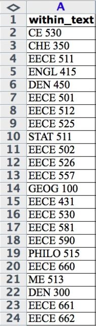The list of cells containing strings of text

The format for the SEARCH function is as follows:

SEARCH(find_text,within_text,start_num)

This is where “find_text” is the string of text you are looking for inside “within_text” and “start_num” is the character number in “within_text,” at which you want to start searching (the default is 1).  The SEARCH function returns a 1 if the string is found in the within_text but if it is NOT found, it returns #VALUE! error, and that is where we run into issues.  For example:

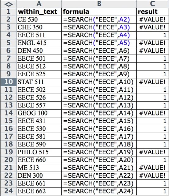Whenever the text is not found in the cell, you get a #VALUE! result

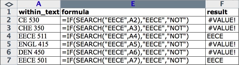
If you are using the search function inside an IF statement, the #VALUE! blows the formula up and you only get results if the result is 1.  Here is how it works out in the data above:

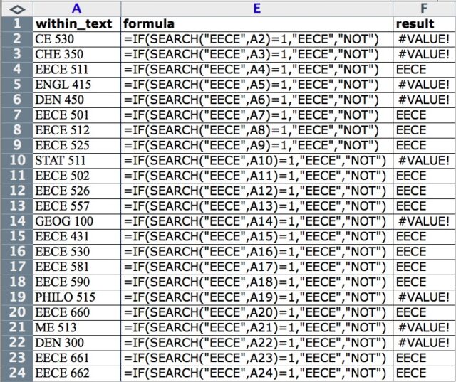The IF function cannot handle the #VALUE! result and fails if the text is not found in the cell

NOTE: it is unnecessary to put the =1 in the IF statements above (and adds unnecessary code).  You can simply put SEARCH(“EECE”,A2) and it will return a positive if it finds the text.  I didn’t realize that till later and corrected it as I went forward.

The only time you get a result is if the cell contains EECE, but if it doesn’t, the IF function fails to give the ELSE result, and here is where the SEARCH function breaks down.  I don’t know why Microsoft created a function that only works when it has a positive result but doesn’t give a 0 for a negative result.  There is a way to get around this though, it’s through another Excel function called ISERROR.  ISERROR returns the logical value TRUE if value refers to any error value, such as #N/A, #VALUE!, #REF!, #DIV/0!, #NUM!, #NAME?, or #NULL!; otherwise, it returns FALSE.  Applied to our situation above, this is what we get:

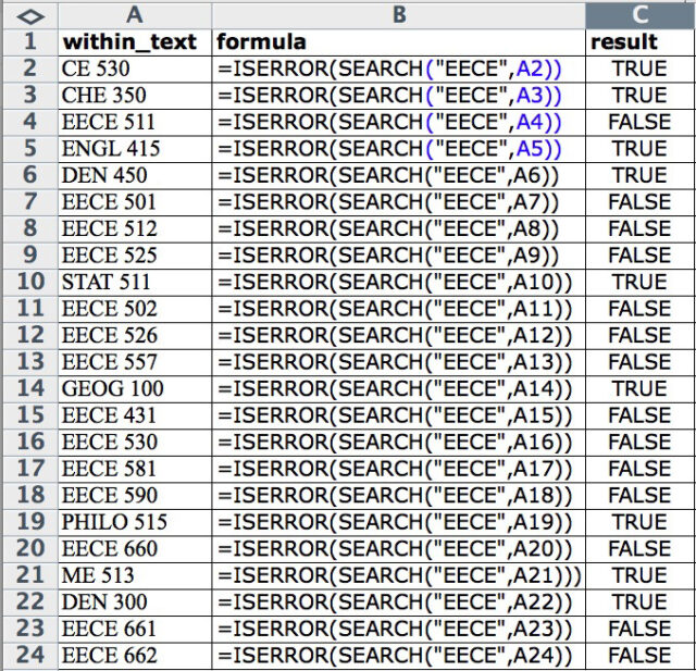The ISERROR function will allow us to get an inverted boolean result without errors when the text is not found

The problem now is that the “result” is opposite of what we actually want, but we can invert it by using the NOT function and achieve the result we wanted in the beginning: getting a TRUE if EECE is contained in the cell and a FALSE if it is not:

Correcting the result with the NOT function

Finally, we can insert this formula into our original IF statement to get the desired results, regardless if the cell contains EECE or not:

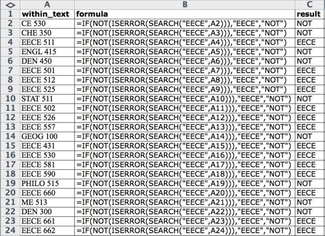Now we get the correct results for the THEN and ELSE results!